

Kush is a Sales Analyst at a distribution company in Pune. Every Friday, he sends a performance report to the Regional Director. He has been using VLOOKUP for two years without any issues – until the day his IT team reorganised the master data sheet and inserted a new column between columns B and C. On Monday morning, Kush opens his report. Every single VLOOKUP cell shows the wrong number.
His formula was pointing to column 3 – which was now “City” instead of “Sales Amount”. His report went to the Director with completely wrong data. The Director called. It was not a pleasant conversation. Kush did not know that there was a formula that would never have broken – regardless of how many columns were added or moved. That formula is INDEX MATCH. You are about to learn it completely.
VLOOKUP is probably the most famous Excel formula. Millions of people use it every day. But it has real, painful limitations – and experienced Excel users quietly moved on from it years ago. INDEX MATCH is what they moved to. It is more flexible, more powerful, more reliable, and once you understand how it works, it is just as easy to write.
This guide will build your understanding from the ground up. You will learn what INDEX and MATCH do individually, how they work together as one powerful combination, how that combination beats VLOOKUP in every meaningful way, and ten practical examples you can use in your actual work today.
Part 1: Understanding INDEX – The ‘Go Fetch’ Function
The Office Filing Cabinet: Think of INDEX like an office filing cabinet. Each drawer is a row. Each folder inside the drawer is a column. You tell the assistant: “Go to drawer 3, take out folder 2.” They bring you exactly that item. You did not describe what was inside. You just gave the position – row number, column number – and INDEX brings back whatever is sitting there.
In Excel, INDEX returns the value of a cell at a specific row and column position inside a range you define. Nothing more, nothing less.
INDEX Syntax:
=INDEX( array, row_num, [col_num] )

  array    → The range of cells you want to look inside
  row_num  → The row number inside that range (1 = first row)
  col_num  → The column number inside that range (optional)
Simple INDEX Example
Suppose you have a table of employee data in the range A1:C10. You want to know what is in row 4, column 2 of that table.
Cell E2:
=INDEX(A1:C10, 4, 2)
Excel goes to row 4 of A1:C10 (which is row 4 of your sheet if your table starts at row 1), and returns whatever is in the second column. That is it. INDEX does not search for anything. It just retrieves a value at a position you specify.
| Cell | Lookup Value | Formula | Excel Returns |
| E2 | Row 4, Col 2 | =INDEX(A1:C10, 4, 2) | Priya Mehta |
| E3 | Row 7, Col 3 | =INDEX(A1:C10, 7, 3) | Finance |
| E4 | Row 2, Col 1 | =INDEX(A1:C10, 2, 1) | 1002 |
Use INDEX on a Single Column for Simpler Formulas: When your return range is a single column – like B1:B100 – you can skip the col_num argument entirely. =INDEX(B1:B100, 5) returns whatever is in the 5th row of that column. This is the most common way INDEX is used inside INDEX MATCH.
Part 2: Understanding MATCH – The ‘Find the Position’ Function
The Office Register: Now picture a different assistant. This one does not fetch anything. Instead, their job is to look through the attendance register and tell you: “Which row number is Ravi Sharma on?” You give them a name, they scan the register from top to bottom, find the match, and report back a number – the row position. That is exactly what MATCH does. It returns the position (the number) of a value inside a list – not the value itself.
MATCH searches for a value inside a range and returns the row number (or column number) where it found that value. It returns a position – a number – not the actual cell value.
MATCH Syntax:
=MATCH( lookup_value, lookup_array, match_type )

  lookup_value  → The value you are searching for
  lookup_array  → The single row or column you are searching in
  match_type    → 0 = exact match (use this almost always)
                  1 = less than or equal (sorted ascending)
                 -1 = greater than or equal (sorted descending)
Simple MATCH Example
You have employee IDs in column A (A2:A11). You want to find the position of employee ID 1005 inside that list.
Cell D2:
=MATCH(1005, A2:A11, 0)
Excel scans A2:A11 from top to bottom, finds 1005, and returns its position number. If 1005 is the 4th item in that range, MATCH returns 4.
| Cell | Lookup Value | Formula | Excel Returns |
| D2 | 1005 | =MATCH(1005, A2:A11, 0) | 4 |
| D3 | “Priya” | =MATCH(“Priya”, B2:B11, 0) | 2 |
| D4 | “Finance” | =MATCH(“Finance”, C2:C11, 0) | 6 |
MATCH Returns a Position, Not a Value: This is the most important concept to remember. MATCH never gives you the actual data – it gives you a number (the row position). That number is exactly what INDEX needs. This is why they work so perfectly together: MATCH finds WHERE the value is, and INDEX goes to THAT position and brings back whatever you want from another column.
Part 3: The Magic Combination – INDEX MATCH Together
Two Assistants, One Perfect Team: You have two assistants now. The first one (MATCH) scans the attendance register: “Ravi Sharma is in row 4.” The second one (INDEX) goes to the filing cabinet: “Row 4, bring me the contents of folder 3 – which is his Salary.” Between them, they can find any piece of information in any table, in any direction. You just have to tell them what to look for and where to bring it from.
When you combine them, MATCH’s output (the row position number) becomes INDEX’s row_num input. INDEX uses that position number to fetch the value from your return column. The result is a complete, dynamic, crash-proof lookup formula.
INDEX MATCH - Combined Formula Structure:
=INDEX( return_column, MATCH( lookup_value, lookup_column, 0 ) )

  return_column  → The column you want to retrieve data FROM
  lookup_value   → What you are searching for (a name, ID, code...)
  lookup_column  → The column you are searching IN
  0              → Always use 0 for exact match
Reading It Like a Sentence
The best way to understand this formula is to read it from the inside out:
- Inside (MATCH): Find the row position of the lookup value inside the lookup column.
- Outside (INDEX): Go to that row position inside the return column and bring back the value sitting there.
Here is how this plays out with a real table. Suppose your data looks like this:
| Column A | Column B | Column C | Column D |
| Emp ID | Employee Name | Department | Salary |
| 1001 | Ravi Sharma | Sales | 42,000 |
| 1002 | Priya Mehta | HR | 38,500 |
| 1003 | Arjun Patel | Operations | 45,000 |
| 1004 | Sneha Joshi | Finance | 51,000 |
| 1005 | Karan Shah | Sales | 39,000 |
You want to look up employee ID 1004 and return their Department from column C. Here is the INDEX MATCH formula:
Cell F2 - Find Department for Emp ID 1004:
=INDEX(C2:C6, MATCH(1004, A2:A6, 0))

Step 1 → MATCH(1004, A2:A6, 0)  returns  4   (1004 is the 4th item in A2:A6)
Step 2 → INDEX(C2:C6, 4) returns Finance (4th item in C2:C6)| Cell | Lookup Value | Formula | Excel Returns |
| F2 | 1004 | =INDEX(C2:C6, MATCH(1004,A2:A6,0)) | Finance |
| F3 | 1002 | =INDEX(C2:C6, MATCH(1002,A2:A6,0)) | HR |
| F4 | 1005 | =INDEX(D2:D6, MATCH(1005,A2:A6,0)) | 39,000 |
| F5 | 1003 | =INDEX(B2:B6, MATCH(1003,A2:A6,0)) | Arjun Patel |
Change Only the Return Column to Get Different Data: Notice how in the table above, the only thing that changes between the formulas is the return column – C2:C6 for Department, D2:D6 for Salary, B2:B6 for Name. The MATCH part stays exactly the same. This makes INDEX MATCH incredibly easy to adapt once you have written it once.
Part 4: Why INDEX MATCH Beats VLOOKUP – 7 Real Reasons
Now that you understand how INDEX MATCH works, let us look at exactly why it is better than VLOOKUP – not just as an opinion, but with specific, practical reasons that affect real work.
Reason 1 – INDEX MATCH Never Breaks When Columns Are Added or Deleted
This is the exact problem that burned Kush in our opening story. VLOOKUP uses a column index number – col_index_num – to find the return column. The moment someone inserts a new column into your table, that index number shifts and your formula starts returning the wrong data. You may not even notice until a Director calls.
Quick Compare: The Critical Difference
VLOOKUP: =VLOOKUP(A2, B:F, 3, FALSE)  ← '3' breaks if a column is inserted INDEX MATCH: =INDEX(D:D, MATCH(A2,B:B,0))  ← references the column directly, never breaks
Reason 2 – INDEX MATCH Can Look to the LEFT
VLOOKUP can only look to the right. Your lookup column must be to the left of your return column. This forces you to rearrange data or use complex workarounds whenever your lookup column is to the right of the data you need.
INDEX MATCH has no such restriction. The lookup column and return column can be in any order – left, right, or the same column. This alone saves significant time when working with real-world data that was not designed with VLOOKUP in mind.
Left Lookup - VLOOKUP Cannot Do This, INDEX MATCH Can:
Data:  Column A = Department | Column B = Emp ID | Column C = Salary
Goal:  Look up Emp ID 1003 and return the Department (which is to the LEFT)

VLOOKUP: IMPOSSIBLE - cannot look left
INDEX MATCH: =INDEX(A2:A100, MATCH(1003, B2:B100, 0))  ← works perfectly
Reason 3 – INDEX MATCH Handles Very Large Datasets Faster
VLOOKUP scans the entire specified table range – every column, even the ones you do not need. INDEX MATCH scans only the lookup column (in MATCH) and the return column (in INDEX). For tables with 50,000+ rows or many columns, this performance difference becomes noticeable.
Reason 4 – INDEX MATCH Finds the Last Match in a List
VLOOKUP always returns the first match it finds. If the same employee appears three times in a list (like a transaction log), VLOOKUP always gets the first entry. INDEX MATCH with a modified MATCH formula can return the last occurrence – extremely useful for audit logs and transaction histories.
Return the LAST Occurrence of a Value:
=INDEX(C2:C1000, MATCH(2, 1/(A2:A1000="EMP1003"), 1))

Note: This is an array formula - press Ctrl+Shift+Enter in older Excel versions
In Excel 365, just press Enter normally
Reason 5 – INDEX MATCH Allows Two-Way Lookups
You can use INDEX MATCH nested inside itself to look up a value at the intersection of a matching row AND a matching column – something VLOOKUP simply cannot do without combining it with MATCH externally.
Reason 6 – INDEX MATCH Is Easier to Audit and Maintain
When you read =INDEX(D2:D100, MATCH(A2, B2:B100, 0)), the formula tells you clearly: ‘Find the value from column D where column B matches A2.’ The formula is self-documenting. VLOOKUP’s column number (the number 4 in =VLOOKUP(A2,B:F,4,FALSE)) tells you nothing about which column it is returning until you count manually.
Reason 7 – INDEX MATCH Works with Dynamic Arrays and Spill
In Excel 365 and Excel 2021, INDEX MATCH integrates cleanly with dynamic array formulas and the new FILTER, SORT, and UNIQUE functions. VLOOKUP is increasingly being left behind in modern Excel workflows.
| Capability | VLOOKUP | INDEX MATCH |
| Look to the left | No | Yes |
| Breaks when columns inserted | Yes – col_index shifts | No – references column directly |
| Returns last match | No – always first | Yes (with array technique) |
| Two-way (row + column) lookup | No | Yes (nested INDEX MATCH) |
| Performance on large data | Slower | Faster (scans only 2 columns) |
| Self-documenting formula | No – col number is cryptic | Yes – column names in formula |
| Works after table restructure | No | Yes |
| Wildcard support | Yes | Yes (with MATCH wildcard) |
| Available in all Excel versions | Yes | Yes |
Part 5: 10 Real-World INDEX MATCH Examples
Here are ten practical examples drawn from real office scenarios. Each one demonstrates a different aspect of INDEX MATCH.
Example 1 – HR: Find Employee Salary by ID
Nisha’s Payroll Query: Nisha in HR gets a call: ‘What is the salary of employee 1047?’ She has 800 rows of data. She does not scroll. She has INDEX MATCH in cell F2.
Cell F2 - Salary Lookup:
=INDEX(D2:D800, MATCH(E2, A2:A800, 0))

  A2:A800 = Employee ID column (lookup column)
  D2:D800 = Salary column (return column)
  E2      = The ID she typed to look up
Example 2 – Sales: Return Product Price from a Price List
Product codes are in column A. Prices are in column C. An order form in column E references product codes and needs to auto-fill the price in column F.
Cell F2 - Price Lookup:
=INDEX(C2:C500, MATCH(E2, A2:A500, 0))
Example 3 – LEFT Lookup: Find Department from Employee Name
Employee names are in column C. Departments are in column A – to the LEFT. VLOOKUP cannot do this.
Cell F2 - Left Lookup:
Data layout:  A = Department | B = Emp ID | C = Employee Name
Goal: Look up name in C, return Department from A

=INDEX(A2:A200, MATCH(E2, C2:C200, 0))
Example 4 – Finance: Map Account Codes to GL Names
Account codes come from an ERP export in column A. You have a reference sheet where column A has codes and column B has full account names. You want to fill in the name beside each code.
Cell B2 - GL Name Lookup:
=INDEX(RefSheet!B2:B500, MATCH(A2, RefSheet!A2:A500, 0))
Example 5 – Operations: Return Warehouse Location by SKU
SKU codes in column A, warehouse locations in column E. A dispatch form needs to auto-fill the warehouse for any SKU entered.
Cell G2 - Warehouse Lookup:
=INDEX(E2:E1000, MATCH(F2, A2:A1000, 0))
Example 6 – Two-Way Lookup: Sales Figure by Region and Month
Meera’s Pivot Problem: Meera’s manager asks: ‘What were North region sales in March?’ The data is a 12×6 grid – months across columns, regions down rows. She needs the value at the intersection of the right row and the right column. This is a two-way lookup – INDEX MATCH inside INDEX MATCH.
Cell F2 - Two-Way Lookup (Region + Month):
=INDEX(B2:M7, MATCH(D2, A2:A7, 0), MATCH(E2, B1:M1, 0))

  B2:M7   = The full data grid (12 months x 6 regions)
  D2      = Region name user types (e.g. 'North')
  A2:A7   = Region name column
  E2      = Month name user types (e.g. 'March')
  B1:M1   = Month header row

First MATCH finds the row. Second MATCH finds the column.
INDEX returns the value at that row-column intersection.
Example 7 – Wildcard Search: Find by Partial Name
If you want to search for a partial name or partial code – for example, any product whose name contains the word ‘Steel’ – use a wildcard (*) with MATCH.
Cell F2 - Wildcard Lookup:
=INDEX(B2:B500, MATCH("*"&E2&"*", A2:A500, 0))

  E2 contains a partial name like: Steel
  The * before and after means 'anything around it'
  MATCH finds the first row where column A contains 'Steel'
Example 8 – Multiple Criteria Lookup (Two Conditions)
You want to look up a row where BOTH the Employee ID AND the Month match your input. This requires an array approach.
Cell G2 - Match Two Conditions (Ctrl+Shift+Enter in older Excel):
=INDEX(D2:D500, MATCH(1, (A2:A500=E2)*(B2:B500=F2), 0))

  A = Employee ID | B = Month | D = Attendance Days
  E2 = The ID you want | F2 = The month you want
  Multiplying two TRUE/FALSE arrays acts like AND logic
  MATCH finds the row where BOTH conditions are 1 (TRUE)
Example 9 – Handle Missing Values Gracefully with IFERROR
If the lookup value does not exist, INDEX MATCH returns an N/A error. Wrap it in IFERROR to show a friendly message instead.
Cell F2 - Clean Error Handling:
=IFERROR(INDEX(C2:C500, MATCH(E2, A2:A500, 0)), "Record Not Found")
Example 10 – Cross-Sheet Lookup
Your data lives on a sheet called ‘MasterData’. Your report is on a different sheet. Reference the other sheet directly inside the formula.
Cell F2 - Cross-Sheet INDEX MATCH:
=IFERROR(INDEX(MasterData!D2:D1000, MATCH(E2, MasterData!A2:A1000, 0)), "Not Found")

  Works exactly the same - just prefix the range with SheetName!
Part 6: Step-by-Step – Building Your First INDEX MATCH
If you want to write your first INDEX MATCH formula right now, follow these five steps. Open any Excel sheet with data before you begin.
- Step 1 – Identify your lookup value. What are you searching for? A name, an ID, a code? This goes inside MATCH as the first argument. Example: the employee ID in cell E2.
- Step 2 – Identify your lookup column. Which column contains the values you are searching in? This is the second argument inside MATCH. Example: the Employee ID column A2:A100.
- Step 3 – Identify your return column. Which column holds the data you want to retrieve? This is the first argument inside INDEX. Example: the Salary column D2:D100.
- Step 4 – Write MATCH first. Start with: =MATCH(E2, A2:A100, 0). Press Enter. Confirm it returns a number (a row position). If it returns #N/A, the lookup value does not exist in the lookup column.
- Step 5 – Wrap it in INDEX. Replace the number with your MATCH formula: =INDEX(D2:D100, MATCH(E2, A2:A100, 0)). Press Enter. You will get the value from the Salary column for that employee.
Write MATCH First, Then Wrap: The most common beginner mistake is trying to write INDEX MATCH all at once and getting confused. Always write and test the MATCH formula first. Confirm it returns the correct row number. Then wrap it inside INDEX. Two small steps is always easier than one big confused step.
Part 7: Common Mistakes and How to Fix Them
| Mistake | What Happens | How to Fix It |
| Using 1 instead of 0 in MATCH | Returns approximate match – wrong data for unsorted lists | Always use 0 as the third MATCH argument for exact match |
| Mismatched range sizes | INDEX gets a position that falls outside the return column | Make sure INDEX range and MATCH range cover the same number of rows |
| Lookup value has extra spaces | MATCH returns #N/A even though the value appears to exist | Use TRIM: MATCH(TRIM(E2), A2:A100, 0) to strip spaces from lookup value |
| Lookup column has mixed data types | MATCH returns #N/A – e.g., IDs stored as text vs numbers | Check and standardise: convert all IDs to the same type (text or number) |
| Forgetting IFERROR | Formula shows ugly #N/A when value is missing | Wrap entire formula: =IFERROR(INDEX(…MATCH(…)),”Not Found”) |
| Cross-sheet range not absolute | When copying formula, sheet reference shifts incorrectly | Lock ranges with $: MasterData!$A$2:$A$1000 prevents shifting |
| Wrong column in return range | Returns data from unexpected column | Double-check that your INDEX range is the correct column, not adjacent one |
| Array formula not entered correctly | Formula shows wrong result or plain text in older Excel | For multi-criteria formulas in Excel 2016/2019, press Ctrl+Shift+Enter |
The Silent Wrong Answer is Worse Than an Error: A formula that returns #N/A is actually easier to catch than one that quietly returns the wrong data. The most dangerous mistake is using MATCH with match_type 1 (approximate) on unsorted data. It will return a wrong value with no error – just wrong numbers sitting silently in your report. Always double-check with 0 (exact match) unless you are certain your data is sorted.
Part 8: 10 Pro Tips for INDEX MATCH
- Lock your ranges with $ signs. When copying the formula across rows or columns, use absolute references: =INDEX($D$2:$D$100, MATCH(E2, $A$2:$A$100, 0)). The lookup and return ranges must not shift when you copy.
- Use full column references for big tables. =INDEX(D:D, MATCH(E2, A:A, 0)) – using entire columns means you never have to update the range when data grows. Performance impact is minimal on modern Excel.
- Use structured table references. If your data is in an Excel Table (Ctrl+T), reference it as =INDEX(Table1[Salary], MATCH(E2, Table1[EmpID], 0)). The table automatically expands when you add rows.
- Use MATCH alone to check if something exists. =ISNUMBER(MATCH(E2, A2:A100, 0)) returns TRUE if the value exists, FALSE if it does not. Useful for validation checks before running lookups.
- Build a lookup dashboard. Put your lookup value in one input cell and write multiple INDEX MATCH formulas pointing to different columns. Change the single input cell and your entire dashboard updates instantly.
- Test on small data first. Write and verify your INDEX MATCH on a 10-row sample. Once it is correct, update the ranges to cover all rows. Never test a new formula directly on live report data.
- Use MATCH without INDEX to find position only. Sometimes you just need to know which row a value is in – not the value from another column. MATCH alone is perfect for this and is faster than INDEX MATCH.
- Combine with IF for conditional lookups. =IF(E2=””, “”, INDEX(D:D, MATCH(E2, A:A, 0))) – this prevents the formula from running if the lookup cell is empty, keeping your sheet clean.
- Name your ranges for ultra-readable formulas. Use Name Manager (Formulas > Define Name) to name A2:A100 as EmpIDs and D2:D100 as Salaries. Then write: =INDEX(Salaries, MATCH(E2, EmpIDs, 0)). Anyone can read that formula instantly.
- Consider XLOOKUP if you have Excel 365. Microsoft released XLOOKUP in 2021 as a cleaner single-function alternative to both VLOOKUP and INDEX MATCH. But INDEX MATCH works on every Excel version from 2003 onwards – which is why it remains the professional standard.
Frequently Asked Questions
Yes – once you understand the two-step logic (MATCH finds position, INDEX retrieves value), it is no harder than VLOOKUP. The extra few characters you type are worth it because the formula never breaks when your spreadsheet changes.
Yes. INDEX MATCH works on filtered tables and sorted tables without any changes to the formula. MATCH will find the first match in the visible or actual data depending on context.
XLOOKUP is a newer single function (Excel 2021 and Microsoft 365 only) that does what INDEX MATCH does with slightly simpler syntax. INDEX MATCH works on every Excel version back to 2003, making it the universal professional standard. Both are excellent – prefer XLOOKUP on new Excel, use INDEX MATCH for compatibility.
It means MATCH could not find your lookup value in the lookup column. Check: (1) Is the value actually in the lookup column? (2) Are there extra spaces – use TRIM. (3) Are numbers stored as text in one column but as real numbers in the other? Use VALUE() to convert.
In Excel 365, yes – use =INDEX(B2:D100, MATCH(E2, A2:A100, 0), 0) with a 0 as the column number to spill all columns for that row. In older Excel versions, you need a separate INDEX MATCH formula for each column.
Absolutely. INDEX MATCH is commonly nested inside IF, IFERROR, SUM, AVERAGE, and other functions. For example: =IFERROR(INDEX(D:D,MATCH(E2,A:A,0)),0) – this returns 0 instead of an error when the value is not found, making SUM calculations safe.
No – the order matters. INDEX is the outer function. MATCH is nested inside as the row_num argument. Swapping them (MATCH outer, INDEX inner) is not a valid formula. Always: INDEX on the outside, MATCH on the inside.
Summary – Your Complete INDEX MATCH Reference
Kush – Six Months Later: Six months after that painful Monday morning call from his Director, Kush has completely rebuilt his reporting templates. Every lookup formula is now INDEX MATCH with locked column references. When the IT team inserts three new columns in the master data sheet the following quarter, Kush’s formulas do not even blink. His reports are correct. He emails the Director before 9 AM. The call he gets this time is a very different kind.
| Function | What It Does | Formula Pattern |
| INDEX | Returns the value at a specific row/column position in a range | =INDEX(range, row_num, [col_num]) |
| MATCH | Returns the position (row number) of a value in a list | =MATCH(value, range, 0) |
| INDEX MATCH | Finds a value by searching one column and returning from another | =INDEX(return_col, MATCH(lookup, search_col, 0)) |
| INDEX MATCH + IFERROR | Clean lookup with friendly error message | =IFERROR(INDEX(…MATCH(…)),”Not Found”) |
| Two-Way INDEX MATCH | Returns value at row+column intersection | =INDEX(grid, MATCH(row_val,rows,0), MATCH(col_val,cols,0)) |
| Multi-Criteria MATCH | Looks up row matching two conditions simultaneously | =INDEX(col, MATCH(1,(A=v1)*(B=v2),0)) – array formula |
| Wildcard INDEX MATCH | Finds partial text matches with * wildcard | =INDEX(col, MATCH(“*”&val&”*”, search_col, 0)) |
The combination of INDEX and MATCH is one of the most important skills you can build in Excel. It is not just a formula – it is a thinking framework. Once you understand how to separate ‘find the position’ from ‘retrieve the value’, every lookup problem in Excel becomes straightforward.
Free Excel Tools at ibusinessmotivation.com If your Monday mornings still involve manually merging files, cleaning duplicates, or splitting data by region – visit ibusinessmotivation.com. Free browser-based tools that do in 3 minutes what INDEX MATCH cannot: file merging, data cleaning, and worksheet splitting. No VBA, no installation required.