

If you have been using Excel for any length of time, you have almost certainly used VLOOKUP. For decades, VLOOKUP was the go-to function for searching data tables. But Microsoft has replaced it with something far more powerful, flexible, and forgiving – the XLOOKUP function.
This Excel XLOOKUP Function Complete Guide will walk you through everything: what XLOOKUP is, how its syntax works, real-world examples for every skill level, a comparison with VLOOKUP and HLOOKUP, advanced use cases, and common mistakes to avoid. By the end, you will be able to confidently use XLOOKUP in any Excel project – and understand exactly why it is the future of Excel lookups.
What Excel XLOOKUP Function? You Will Learn in This Guide
Syntax and all 6 parameters explained | XLOOKUP vs VLOOKUP vs HLOOKUP | Basic to advanced examples | Exact, approximate, and wildcard matching | Two-way lookups | Error handling | Nested XLOOKUP | Performance tips | Frequently asked questions.
XLOOKUP is a modern lookup function introduced by Microsoft in Excel for Microsoft 365 and Excel 2021. It was designed to overcome nearly every limitation that made VLOOKUP frustrating to use. Unlike VLOOKUP, XLOOKUP can search in any direction, return multiple columns, handle errors natively, and does not break when you insert or delete columns.
In short: XLOOKUP is what VLOOKUP always should have been.
| Feature | VLOOKUP | XLOOKUP |
| Search Direction | Left to right only | Any direction (left, right, up, down) |
| Column Reference | Column index number (fragile) | Direct range reference (robust) |
| Error Handling | Requires IFERROR wrapper | Built-in [if_not_found] argument |
| Return Multiple Columns | No | Yes, with a single formula |
| Default Match Mode | Approximate (can cause errors) | Exact match by default |
| Works with Horizontal Data | No (use HLOOKUP) | Yes, natively |
| Array/Spill Support | No | Yes |
| Performance on Large Data | Slower (scans entire column) | Faster with binary search option |
XLOOKUP Syntax – All 6 Parameters Explained
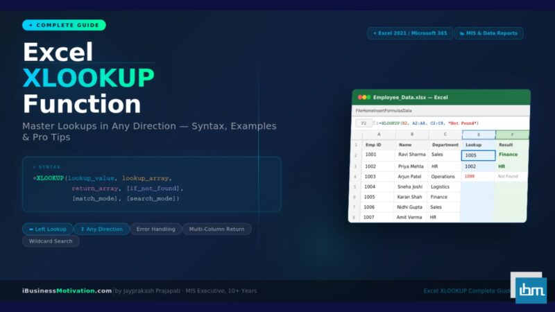
The full syntax of the XLOOKUP function is:
=XLOOKUP(lookup_value, lookup_array, return_array, [if_not_found], [match_mode], [search_mode])The first three arguments are required. The last three are optional but extremely useful. Here is what each one means:
| Argument | Required? | What It Does | Example |
| lookup_value | Yes | The value you are searching for | “Ravi” or A2 or 1001 |
| lookup_array | Yes | The range/column where you want to search | A2:A100 or $A$2:$A$100 |
| return_array | Yes | The range/column to return a value from | B2:B100 or C2:D100 |
| [if_not_found] | No | Text or value returned if no match is found | “Not Found” or 0 |
| [match_mode] | No | Type of match: 0=exact, -1=next smaller, 1=next larger, 2=wildcard | 0 for exact match |
| [search_mode] | No | Search order: 1=first-to-last, -1=last-to-first, 2=binary ascending, -2=binary descending | 1 (default) |
By default (when you omit the last three arguments), XLOOKUP performs an exact match and searches from the first item to the last. This is already safer than VLOOKUP’s default approximate match, which can return wrong results on unsorted data.
Basic XLOOKUP Examples (Perfect for Beginners)
Example 1: Find an Employee’s Department
Scenario: You have a list of employee IDs in column A and their departments in column B. You want to find the department for Employee ID 1042.
=XLOOKUP(1042, A2:A100, B2:B100, "Not Found")This formula searches for 1042 in column A, and returns the corresponding value from column B. If 1042 does not exist, it displays “Not Found” instead of an error.
Example 2: Look Up a Product Price
Scenario: Product names are in column A, prices are in column D. You want to look up a price from a dropdown cell F2.
=XLOOKUP(F2, A2:A500, D2:D500, "Product Not Found")Example 3: Search to the LEFT (Not Possible in VLOOKUP)
Scenario: Employee names are in column C, and their IDs are in column A (to the left). With VLOOKUP, you cannot search column C and return column A. With XLOOKUP, this is simple:
=XLOOKUP("Priya", C2:C100, A2:A100, "Not Found")No column rearranging needed. No INDEX-MATCH workaround required. XLOOKUP handles it directly.
Intermediate XLOOKUP Examples
Example 4: Return Multiple Columns at Once
One of XLOOKUP’s most powerful features is the ability to return multiple columns in a single formula. If you want to retrieve both the department and salary for an employee:
=XLOOKUP(F2, A2:A100, C2:D100, "Not Found")Here, C2:D100 is a two-column return array. Excel will spill the results into two adjacent cells automatically. This eliminates the need to write two separate VLOOKUP formulas.
Example 5: Handle Errors Gracefully
Instead of wrapping your formula in IFERROR like this:
=IFERROR(VLOOKUP(A2, Table1, 2, FALSE), "Not Found")With XLOOKUP, error handling is built right in:
=XLOOKUP(A2, Table1[Name], Table1[Score], "No Record Found")Cleaner, shorter, and easier to read and maintain.
Example 6: Wildcard Search (Partial Matches)
If you want to find a name that contains a specific keyword – for example, any employee whose name contains “Kumar” – set match_mode to 2:
=XLOOKUP("*Kumar*", A2:A100, B2:B100, "Not Found", 2)The asterisks are wildcard characters. The 2 in the match_mode position enables wildcard matching.
Advanced XLOOKUP Techniques
Two-Way Lookup: Find a Value at the Intersection of a Row and Column
A two-way lookup means you search both rows and columns simultaneously. For example, finding the sales figure for a specific region and a specific month. Nested XLOOKUP makes this easy:
=XLOOKUP(F2, A2:A13, XLOOKUP(G2, B1:E1, B2:E13))The inner XLOOKUP finds the correct column (month). The outer XLOOKUP finds the correct row (region). The result is the value at their intersection – no complex array formulas needed.
Last Match Instead of First Match
VLOOKUP always returns the first matching value. But what if you need the most recent entry for a repeated value? Use search_mode -1 to search from the last item:
=XLOOKUP(F2, A2:A100, C2:C100, "Not Found", 0, -1)This is extremely useful for transaction logs, audit trails, or any dataset where the same ID appears multiple times and you want the latest record.
Approximate Match for Salary Bands or Grade Tables
For grade tables or tax slabs where you need the closest match below the lookup value, use match_mode -1:
=XLOOKUP(B2, D2:D10, E2:E10, "Out of Range", -1)Match mode -1 returns the next smaller value if an exact match is not found. This is ideal for commission tiers, tax brackets, and performance bands.
Binary Search for Massive Datasets
For very large sorted datasets (100,000+ rows), standard search can be slow. Set search_mode to 2 (binary ascending) for significantly faster lookups:
=XLOOKUP(F2, A2:A1000000, B2:B1000000, "Not Found", 0, 2)Important: The lookup array must be sorted in ascending order for binary search to return correct results.
Combine XLOOKUP with IF for Conditional Lookups: You can nest XLOOKUP inside IF to return different values based on conditions. For example: =IF(G2=”North”, XLOOKUP(F2, A2:A100, B2:B100), XLOOKUP(F2, A2:A100, C2:C100)) – this returns values from column B for North region and column C for all others.
XLOOKUP vs VLOOKUP vs INDEX-MATCH: A Complete Comparison
Many Excel users ask: should I switch from VLOOKUP to XLOOKUP? Or is INDEX-MATCH still better? Here is a comprehensive comparison to help you decide:
| Criteria | VLOOKUP | INDEX-MATCH | XLOOKUP |
| Ease of use | Easy but limited | Moderate – two functions | Easy and powerful |
| Left lookup | Not possible | Yes | Yes |
| Horizontal lookup | No (use HLOOKUP) | Yes | Yes |
| Insert/delete columns | Breaks formula | Safe | Safe |
| Return multiple columns | No | With array tricks | Yes, natively |
| Built-in error handling | No | No | Yes |
| Wildcard matching | Yes | With MATCH wildcards | Yes |
| Last match search | No | With workarounds | Yes (-1 search mode) |
| Binary search support | No | No | Yes (2x/-2x modes) |
| Formula complexity | Low | High | Low to medium |
| Excel version required | All versions | All versions | Excel 2021 / Microsoft 365 |
Verdict: For Excel 2021 and Microsoft 365 users, XLOOKUP is the clear winner in almost every category. If you are still on older Excel versions, INDEX-MATCH remains the best alternative to VLOOKUP.
Common XLOOKUP Mistakes and How to Avoid Them
| Mistake | Why It Happens | How to Fix It |
| #N/A error returned | No match found and no if_not_found argument set | Always add the 4th argument: “Not Found” or 0 |
| Wrong values returned | lookup_array and return_array are different sizes | Ensure both arrays have exactly the same number of rows |
| Formula returns all #SPILL! errors | A cell in the spill range is not empty | Clear all cells in the spill area |
| Wildcard not working | match_mode not set to 2 | Add 2 as the 5th argument |
| Approximate match giving wrong results | match_mode set incorrectly for unsorted data | Use exact match (0) unless data is sorted |
| Binary search returning incorrect values | Data is not properly sorted | Sort the lookup column before using search_mode 2 |
| XLOOKUP not available in Excel | User is on Excel 2019 or older | Upgrade to Microsoft 365 or use INDEX-MATCH as alternative |
When to Use XLOOKUP: Real-World Scenarios
Here are the most practical use cases where XLOOKUP delivers the most value in day-to-day Excel work:
HR & Payroll
- Looking up employee salary from a master HR sheet
- Finding designation or department based on employee ID
- Retrieving joining date or performance rating
Sales & CRM Reporting
- Matching customer names to their account managers
- Finding the latest order date for a customer (using search_mode -1)
- Pulling product prices or discount rates from a pricing table
Finance & Accounting
- Applying tax slabs or commission brackets with approximate match
- Mapping transaction codes to GL account names
- Looking up currency exchange rates for invoice processing
Operations & Inventory
- Checking stock levels for a specific SKU
- Finding the assigned warehouse for a product category
- Two-way lookup for zone and product intersection in pricing grids
10 Pro Tips to Get the Most from XLOOKUP
- Always lock lookup and return arrays with $ signs if copying the formula across rows or columns.
- Use structured table references like Table1[Column] instead of range references for dynamic, auto-expanding lookups.
- When returning multiple columns, make sure the cells to the right are empty to allow spill.
- For case-sensitive lookups, combine XLOOKUP with EXACT: =XLOOKUP(TRUE, EXACT(F2, A2:A100), B2:B100).
- Use XLOOKUP inside IFERROR as an extra safety net if combining with other formulas that might generate errors.
- To return the last non-blank value in a column, combine XLOOKUP with FILTER.
- For dashboards, pair XLOOKUP with dropdown validation lists in the lookup_value cell to create interactive reports.
- In Power Query, the equivalent of XLOOKUP is a merge query – but for in-sheet lookups, XLOOKUP is faster and simpler.
- Name your lookup ranges using the Name Manager for cleaner, more readable formulas.
- Test XLOOKUP on small data first, confirm accuracy, then apply to full datasets.
Frequently Asked Questions About XLOOKUP
No. XLOOKUP is available only in Excel for Microsoft 365 (subscription), Excel 2021, and Excel for the web. It is not available in Excel 2019, Excel 2016, or any earlier version. If your organization uses older Excel versions, use INDEX-MATCH as the alternative.
Yes. XLOOKUP works both vertically (like VLOOKUP) and horizontally (like HLOOKUP). You simply change the lookup_array and return_array to row ranges instead of column ranges. One function replaces two.
By default, XLOOKUP returns the first matching value. To get the last matching value, set search_mode to -1. To retrieve all matching values, use FILTER function instead.
Yes. Reference another sheet like this: =XLOOKUP(A2, Sheet2!A:A, Sheet2!B:B, “Not Found”). For workbooks: =XLOOKUP(A2, [Workbook2.xlsx]Sheet1!A:A, [Workbook2.xlsx]Sheet1!B:B, “Not Found”).
For standard searches, XLOOKUP and VLOOKUP have similar performance on small datasets. For large datasets with sorted data, XLOOKUP with binary search mode (search_mode 2) is significantly faster than VLOOKUP.
Yes. Set the return_array to a full row range like B2:Z2 and XLOOKUP will return all values in that row, spilling them across columns.
Wrap it with EXACT function: =XLOOKUP(TRUE, EXACT(F2, A2:A100), B2:B100, “Not Found”). EXACT returns TRUE only for exact case matches, and XLOOKUP then finds that TRUE.
Summary: Why XLOOKUP Is the Future of Excel Lookups
XLOOKUP is not just a replacement for VLOOKUP – it is a complete redesign of how lookups work in Excel. It is more flexible, more forgiving, more readable, and more powerful. Once you start using XLOOKUP, you will wonder how you ever managed without it.
To summarize what makes XLOOKUP the definitive lookup function for modern Excel users:
- It searches in any direction – left, right, up, or down
- It handles errors natively without requiring IFERROR wrappers
- It returns multiple columns in a single formula
- It matches exactly by default – no accidental approximate matches
- It supports wildcard, approximate, and binary search modes
- It does not break when columns are inserted or deleted
- It replaces VLOOKUP, HLOOKUP, and complex INDEX-MATCH combinations
Whether you are a beginner building your first lookup formula or a data analyst managing complex reporting workbooks, mastering XLOOKUP will immediately improve both the quality and efficiency of your Excel work.