

Ask most Excel users how to automate repetitive tasks and they will say: learn VBA. Write macros. Code it. But what if you are not a programmer? What if your company locks down macro-enabled files? What if you simply want powerful automation without the complexity of writing code?
The truth is – Excel has become remarkably powerful without VBA. Microsoft has quietly built an entire ecosystem of no-code and low-code automation features directly into Excel. Features like Power Query, Flash Fill, dynamic arrays, conditional formatting rules, data validation, and named ranges can replace or eliminate dozens of manual, repetitive tasks that users currently do by hand every day.
This guide is your complete introduction to Excel automation without VBA. You will learn every major no-code automation feature, see real examples for each one, and walk away with practical tools you can use immediately – without writing a single line of code.
Section 1: Why You Do Not Need VBA to Automate Excel
VBA (Visual Basic for Applications) is a programming language that has powered Excel automation since 1993. It is incredibly powerful – but it comes with real limitations that make it unsuitable for many users and organizations.
| VBA Limitation | The Problem It Creates |
| Requires coding knowledge | Most Excel users are not programmers – VBA has a steep learning curve |
| Security restrictions | Many IT departments disable macros company-wide for security reasons |
| File format dependency | VBA files must be saved as .xlsm – standard .xlsx files cannot contain macros |
| Breaks across Excel versions | Macros written in one Excel version can fail or behave differently in another |
| Not available in Excel Online | VBA does not run in browser-based Excel or on mobile devices |
| Maintenance burden | When processes change, someone with coding knowledge must update the macro |
Every limitation above is solved by no-code automation features. Power Query works in Excel Online. Flash Fill works on every device. Dynamic arrays are version-independent. Conditional formatting rules require zero maintenance. This is why learning no-code automation is not just easier – in many situations, it is actually the smarter choice.
| Automation Need | No-Code Excel Feature | What It Replaces |
| Import and clean data from multiple sources | Power Query | VBA data import macros |
| Fill patterns in data instantly | Flash Fill | VBA string manipulation macros |
| Auto-highlight important rows | Conditional Formatting | VBA cell coloring loops |
| Prevent wrong data entry | Data Validation | VBA input validation macros |
| Dynamic calculations that auto-expand | Dynamic Arrays (FILTER, SORT, UNIQUE) | VBA array formulas |
| Consistent, structured data ranges | Excel Tables | VBA range management |
| Merge, split, clean files online | Browser-based Excel Tools | Entire macro workflows |
Section 2: Power Query – The Most Powerful No-Code Feature in Excel
If you learn only one no-code automation feature from this entire guide, make it Power Query. Power Query is a data transformation and automation engine built directly into Excel (available since Excel 2016, and in earlier versions as an add-in). It can replace hours of manual data work with a reusable, one-click refresh process.
What Power Query Does
- Imports data from Excel files, CSV files, databases, web pages, SharePoint, and more
- Cleans data: removes duplicates, fixes formatting, fills blanks, splits columns, changes data types
- Merges and appends multiple tables from different files into one clean master table
- Transforms data: pivots, unpivots, groups, aggregates, and reshapes tables
- Remembers every step – one click refreshes the entire process with new data
Real Example: Merging 5 Monthly Sales Files into One Annual Report
Before Power Query: you would manually open each of the 12 monthly files, copy the data, paste it into a master sheet, clean the formatting inconsistencies, remove duplicates, and format the final output. This takes 60 to 90 minutes every month.
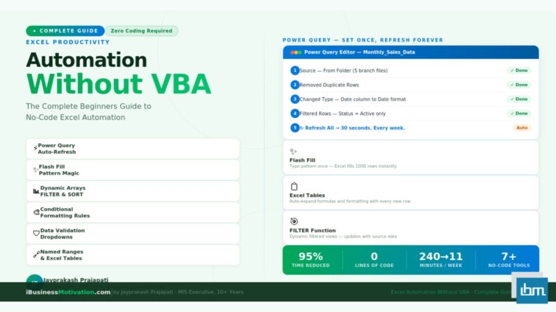
With Power Query: you set up the query once. Every month, you drop the new file into the same folder and click Refresh. Power Query imports, cleans, and merges everything automatically in under 30 seconds.
How to Get Started with Power Query (Step by Step)
- Click the Data tab in the Excel ribbon.
- Click Get Data (or Get & Transform Data depending on your Excel version).
- Choose your data source – From File > From Workbook, or From Text/CSV, or From Web.
- Select your file and click Transform Data. The Power Query Editor opens.
- Apply transformations: remove columns, change data types, filter rows, merge tables.
- Click Close & Load. Your clean data loads into a new Excel sheet.
- Next time your source data updates, click Data > Refresh All. Done.
| Power Query Task | Manual Time | With Power Query | Time Saved |
| Merge 5 department files | 75 minutes | First setup: 15 min | Monthly: 30 sec | 74+ minutes every month |
| Clean duplicates and blanks | 65 minutes | Apply Remove Duplicates step once | 65 minutes every run |
| Change all date formats | 45 minutes | Change Type step applied once | 45 minutes every run |
| Unpivot monthly columns to rows | 90 minutes | Unpivot Columns in one click | 90 minutes every run |
| Filter and keep only specific rows | 30 minutes | Filter Rows step applied automatically | 30 minutes every run |
Section 3: Flash Fill – Instant Pattern Recognition Automation
Flash Fill is one of the simplest and most satisfying automation features in Excel. It watches what you type, recognizes the pattern, and fills in the rest of the column automatically. No formulas. No code. No setup.
Flash Fill was introduced in Excel 2013 and works in all Excel versions from 2013 onward, including Excel for Microsoft 365.
How Flash Fill Works
- You have raw data in column A that needs to be transformed.
- Click on cell B1 – the column next to your data.
- Type the transformed version of the first cell exactly as you want it.
- Start typing in B2. Excel detects the pattern and shows a preview in gray.
- Press Enter to accept, or press Ctrl+E to trigger Flash Fill manually.
| Use Case | Raw Data (Column A) | Flash Fill Result (Column B) | What It Did |
| Extract first name | Ravi Sharma | Ravi | Split text before the space |
| Extract last name | Priya Mehta | Mehta | Split text after the space |
| Combine first + last | Ravi | Sharma (two cols) | Ravi Sharma | Merged two columns |
| Format phone numbers | 9876543210 | (987) 654-3210 | Reformatted number pattern |
| Extract domain from email | ravi@company.com | company.com | Extracted text after @ |
| Capitalize names properly | rAVI sHARMA | Ravi Sharma | Fixed capitalization pattern |
| Extract year from date text | Invoice_2024_001 | 2024 | Extracted numeric pattern |
Section 4: Excel Tables – Automation You Set Up Once and Forget
Converting a plain data range into an Excel Table (Insert > Table, or Ctrl+T) is one of the most underused automation features in Excel. It seems like a simple formatting change – but it is actually a structural upgrade that automates several things simultaneously.
What Excel Tables Automate Automatically
- Auto-expanding ranges: When you add a new row to the bottom of a table, all formulas, formatting, data validation rules, and conditional formatting rules in that table automatically extend to include the new row. You never need to copy-paste formats or drag formulas down again.
- Structured references: Instead of writing =SUM(C2:C500), you write =SUM(Table1[Sales]). This reference always covers the entire column, no matter how many rows exist. No more updating formula ranges when your data grows.
- Auto-filter headers: Every table automatically gets filter dropdowns on every column header. No setup needed.
- Total row: Right-click the table and enable the Total Row. Excel adds a smart total row with SUM, AVERAGE, COUNT and more – and it stays at the bottom even as rows are added.
- Consistent formatting: Banded row colors, header styling, and borders are maintained automatically as rows are added or deleted.
Section 5: Dynamic Arrays – Formulas That Automate Entire Reports
Dynamic Array functions were introduced in Excel for Microsoft 365 and Excel 2021. They are single formulas that automatically spill their results across multiple cells – creating entire filtered lists, sorted tables, or unique value summaries with one formula.
These functions replace what previously required complex array formulas, helper columns, or VBA loops to accomplish.
| Function | What It Does | Example Use Case |
| FILTER | Returns only rows that match a condition | Show only North region sales from a master table |
| SORT | Returns a sorted version of a range | Display top performers ranked by sales value |
| SORTBY | Sorts by another column or array | Sort employee list by department then by salary |
| UNIQUE | Returns only unique values from a range | Get a list of all distinct departments or regions |
| SEQUENCE | Generates a sequence of numbers | Auto-number rows or create date series |
| RANDARRAY | Fills a range with random numbers | Generate test data or random samples |
Real Example: Auto-Filtering a Report by Region
Imagine a master sales table with 500 rows across North, South, East, and West regions. Previously, you would manually filter the table, copy the visible rows to a new sheet, and format it. You would do this every week.
With the FILTER function, you write a single formula on a separate sheet:
=FILTER(SalesData, SalesData[Region]="North", "No North data found")This formula automatically returns every North region row. When the master data is updated, the filtered view updates instantly without any manual work. No copying. No filtering. No separate process.
Real Example: Instant Unique Department List
=UNIQUE(EmployeeTable[Department])This single formula returns every unique department name from your employee table. As new departments are added to the data, the list updates automatically. This is what previously required Remove Duplicates or a complex COUNTIF-based helper column.
Section 6: Conditional Formatting – Visual Automation
Conditional Formatting is automation for your eyes. Instead of manually scanning rows to find important values, Conditional Formatting automatically highlights cells, applies color scales, or adds icons based on rules you set once. Every time your data changes, the formatting updates automatically.
Most Useful Conditional Formatting Rules for Automation
| Rule Type | What It Does Automatically | Best Use Case |
| Highlight Cells Rules | Colors cells above, below, equal to, or between thresholds | Flag salaries above budget, overdue dates, zero stock |
| Top/Bottom Rules | Highlights top 10%, bottom 10%, above/below average | Instantly spot best and worst performers |
| Data Bars | Adds a progress-bar style bar inside each cell | Visual comparison of sales across regions |
| Color Scales | Applies a gradient from low to high values | Heatmap of performance data across departments |
| Icon Sets | Adds traffic light or arrow icons based on value | Status indicators for project tracking |
| Formula-Based Rules | Applies formatting to entire rows based on any condition | Highlight entire row if Status = Overdue |
Advanced Tip: Formula-Based Row Highlighting
The most powerful conditional formatting rule uses a custom formula to highlight entire rows. For example, to automatically highlight every row where the Status column says Overdue in red:
- Select your entire data range (e.g., A2:F200).
- Go to Home > Conditional Formatting > New Rule.
- Select Use a formula to determine which cells to format.
- Enter the formula: =$F2=”Overdue” (lock the column with $, leave row relative).
- Set the fill color to red and click OK.
Now every row where column F says Overdue is automatically highlighted in red. When the status changes to Complete, the red highlighting disappears automatically. This is dynamic visual automation with zero code.
Section 7: Data Validation – Automate Error Prevention at the Source
Most Excel automation focuses on processing data after it has been entered. Data Validation takes a different approach: it prevents incorrect data from being entered in the first place. This is one of the most powerful and underused automation strategies available to beginners.
Types of Data Validation Rules
| Validation Type | What It Prevents | Example |
| Whole Number | Non-integers and numbers outside a range | Age must be between 18 and 65 |
| Decimal | Numbers outside a decimal range | Discount must be between 0 and 0.50 |
| List | Any value not in a predefined list | Region must be North, South, East, or West |
| Date | Dates outside an allowed range | Joining date cannot be before 2010 |
| Text Length | Text that is too short or too long | Employee ID must be exactly 6 characters |
| Custom Formula | Any condition you can express as a formula | End date must be after Start date |
Dropdown Lists: The Most Commonly Used Validation
Dropdown validation is one of the most practical no-code automation features for data entry forms. Instead of users typing department names, region names, or status values (and making spelling mistakes), they select from a controlled list.
- Select the cells where you want the dropdown.
- Go to Data > Data Validation.
- Under Allow, select List.
- In the Source field, type your options separated by commas: North,South,East,West – or reference a named range like =DepartmentList.
- Click OK. Every selected cell now has a dropdown arrow.
Section 8: Named Ranges and Named Tables – Clean, Maintainable Automation
Named Ranges let you give a meaningful name to a cell or range of cells. Instead of referencing =SUM(C2:C150), you write =SUM(MonthlySales). This is not just a readability improvement – it fundamentally changes how maintainable and automatable your workbook becomes.
| Instead of This Formula | Write This with Named Ranges | Why It Is Better |
| =VLOOKUP(A2,C2:F200,3,FALSE) | =VLOOKUP(A2,EmployeeTable,3,FALSE) | If the table moves, the formula still works |
| =SUM(D2:D1000) | =SUM(AnnualSales) | Self-documenting – anyone can read it |
| =IF(B2>5000,”Senior”,”Junior”) | =IF(B2>SeniorThreshold,”Senior”,”Junior”) | Change the threshold in one cell, all formulas update |
| =AVERAGE(F2:F100) | =AVERAGE(PerformanceScores) | Works even if rows are added or removed |
How to Create a Named Range
- Select the cell or range you want to name.
- Click in the Name Box (the box showing the cell address, top-left corner of Excel).
- Type your chosen name (no spaces – use underscores: Monthly_Sales).
- Press Enter. The name is now saved.
- Use this name in any formula anywhere in the workbook.
For a centralized view of all named ranges, go to Formulas > Name Manager. You can edit, delete, or update any named range from this single location.
Section 9: Browser-Based Excel Tools – The Fastest No-Code Automation
| Tool | What It Automates | Time Before | Time After |
| Multiple Excel File Merger | Merge 2-20 Excel files into one master file | 75 minutes manual | 3 minutes |
| Excel Data Cleaner | Remove duplicates, blank rows, fix formatting in one pass | 65 minutes manual | 2 minutes |
| Excel Worksheet Split Tool | Split one file into separate files by column value | 55 minutes manual | 4 minutes |
| CSV to Excel Converter | Convert and clean CSV files for Excel use | 20 minutes manual | 1 minute |
Real Case Study: 4 Hours to 11 Minutes
A documented MIS workflow at a mid-sized company in Ahmedabad involved merging 5 department files, cleaning duplicates, and splitting by region every Monday morning. The manual process took 240 minutes (4 hours) per week with a 75% error rate. After replacing the process with browser-based tools from ibusinessmotivation.com, the same workflow now takes 11 minutes – a 95.4% time reduction – with zero errors. No VBA. No Excel setup. No technical skills required.
Section 10: Putting It All Together – A Real No-Code Automated Workflow
Knowing individual features is valuable. But the real power comes from combining them into a complete automated workflow. Here is a real-world example that shows how five no-code features work together to fully automate a weekly HR reporting process.
The Scenario: Weekly HR Department Report
Every Friday, an HR team receives salary and attendance data from 6 branch offices in separate Excel files. They need to merge the data, clean it, produce a summary by department, highlight overdue performance reviews, and send each branch head their own file. Manually, this takes 3.5 hours.
The No-Code Automated Solution
| Step | Task | No-Code Tool Used | Time |
| 1 | Merge 6 branch files into one master file | Browser-based File Merger Tool | 3 minutes |
| 2 | Remove duplicates and fix blank rows | Browser-based Data Cleaner Tool | 2 minutes |
| 3 | Import master file and apply transformations | Power Query (Refresh All) | 1 minute |
| 4 | Auto-generate department summary | UNIQUE + SUMIF formulas in Excel Table | Automatic |
| 5 | Highlight overdue reviews in red | Conditional Formatting formula rule | Automatic |
| 6 | Validate all new entries for correct department names | Data Validation dropdown lists | Automatic |
| 7 | Split master file by branch for individual emails | Browser-based Worksheet Split Tool | 4 minutes |
Total time after automation: 10 minutes. Time saved per week: 200 minutes. VBA code written: Zero lines. Every tool and feature in this workflow is available to you right now, for free. Power Query is built into Excel 2016+. Dynamic array formulas are in Microsoft 365. Conditional formatting is in every Excel version since 2007. Browser-based tools at ibusinessmotivation.com work on any device with a browser.
Section 11: Choosing the Right No-Code Automation Feature
With so many tools available, beginners often ask: which feature should I use for my specific problem? Here is a practical decision guide.
| Your Problem | Best No-Code Solution | Why |
| I manually import and clean data every week | Power Query | Set up once, refresh in one click forever |
| I need to reformat names, emails, or codes | Flash Fill | Instant pattern recognition, zero formulas |
| My data range keeps growing and breaking formulas | Excel Tables | Tables auto-expand all formulas and formatting |
| I need filtered views that update automatically | FILTER function (Dynamic Arrays) | Formula-based – updates with source data |
| I want to highlight important rows automatically | Conditional Formatting | Rule-based – updates as values change |
| People keep entering wrong values | Data Validation | Prevents errors at the source |
| I need to merge or split Excel files quickly | Browser-based Tools | No setup, works on any device |
| My formulas are confusing and hard to maintain | Named Ranges | Makes formulas readable and portable |
| I need unique values or sorted lists auto-generated | UNIQUE and SORT functions | Single formula, auto-updates |
Section 12: Common No-Code Automation Mistakes to Avoid
| Mistake | The Problem | The Fix |
| Using plain ranges instead of Excel Tables | Formulas break when rows are added | Always convert data to a Table with Ctrl+T first |
| Not naming Power Query steps | Queries become impossible to read and maintain | Double-click each step in the Applied Steps panel to give it a descriptive name |
| Flash Fill on a small sample | Pattern is not recognized correctly | Provide 2-3 examples before triggering Flash Fill |
| Applying conditional formatting to too many cells | Workbook becomes slow and laggy | Apply rules only to the exact range needed, not entire columns |
| Hard-coding values in formulas | Single change requires updating many formulas | Store values in named cells and reference those names |
| Not testing Data Validation with bad data | Users find workarounds or paste over validation | Test by pasting invalid data – ensure validation blocks it |
| Forgetting to Refresh Power Query | Report shows stale data from last refresh | Set up automatic refresh: Data > Queries & Connections > Properties > Refresh on file open |
Frequently Asked Questions
Absolutely. Power Query, Flash Fill, Excel Tables, dynamic array functions, conditional formatting, and data validation are all entirely visual and menu-driven. None of them require writing code. Millions of professionals use these features every day without any programming background.
Power Query has a learning curve, but it is significantly gentler than VBA. Most beginners can complete their first useful query – importing and cleaning a CSV file – within one hour of starting. The visual Applied Steps panel shows exactly what the query is doing at each stage, which makes it easy to understand and modify.
No. FILTER, SORT, SORTBY, UNIQUE, SEQUENCE, and RANDARRAY are available only in Excel for Microsoft 365 and Excel 2021. They are not available in Excel 2019, 2016, or earlier. For older versions, use Power Query or INDEX/MATCH-based approaches for similar results.
Free tiers of browser-based tools typically handle files up to 2MB, which covers most standard business Excel files. Premium plans handle larger files. For files with hundreds of thousands of rows, Power Query inside Excel is generally the better choice for large-scale data processing.
Python and Power Automate are more powerful but require significantly more technical setup and knowledge. The features in this guide require only Excel and a web browser – no additional software, no APIs, no programming environments. For most standard business reporting and data processing tasks, the no-code features covered here are more than sufficient.
Most features work in Excel Online, including Excel Tables, conditional formatting, data validation, dynamic array functions, and basic Power Query. Some advanced Power Query connectors and transformations require the desktop version. Flash Fill is available in the desktop version only.
Start with Excel Tables and Conditional Formatting – they require zero learning curve and immediately improve any existing workbook. Then learn Flash Fill for instant text transformations. Next, invest 1-2 hours in Power Query – it will pay dividends every week for years. Finally, explore dynamic array functions to replace manual filtering and sorting tasks.
Your No-Code Excel Automation Learning Roadmap
| Week | Focus Area | What to Practice | Time Investment |
| Week 1 | Excel Tables + Conditional Formatting | Convert one existing data range to a Table. Add one conditional formatting rule. | 2 hours |
| Week 2 | Flash Fill + Data Validation | Use Flash Fill on a name or email column. Add a dropdown list to a data entry form. | 2 hours |
| Week 3 | Power Query Basics | Import one CSV file with Power Query. Apply Remove Duplicates and Change Type steps. | 3 hours |
| Week 4 | Dynamic Arrays | Write a FILTER formula and a UNIQUE formula on a real dataset. | 2 hours |
| Week 5 | Full Workflow | Automate one real recurring task end-to-end using at least 3 of the above features. | 3 hours |
The total investment is roughly 12 hours across five weeks. The return on that investment – in time saved on repetitive Excel work – will be measured in hours per month, every month, for your entire career.
Free Tools at ibusinessmotivation.com For instant no-code file automation – merging Excel files, cleaning data, splitting by region – visit ibusinessmotivation.com. All tools are free for files up to 2MB with no signup required. Use them alongside the Excel built-in features covered in this guide for a complete no-code automation stack.